Friday 6 January 2017

A Final Word

As you might expect, every series eventually reaches its end. I’m very proud to have had the opportunity to discuss such an overlooked property of our atmosphere. It’s always nice to experience the subtleties in our surroundings, regardless of how dynamic or prevalent they may be. 

I’d like to thank anyone who took the time to read through any of the blogs and hope you’ve at least had a chance to broaden your perspective on what you may have never otherwise ever heard about. To any new readers, I encourage you to have a browse of what the series has to offer as it was designed from scratch to cater to anyone, assuming you read them in order. 

It has truly been a pleasure and I sincerely hope that someone may have benefited, even if only very slightly from my interpretations of one of the most overlooked atmospheric phenomena. To be so close and yet know so little is a poor state to be in. 


Until further notice, I bid you all a farewell!

-Muwaffaq


Monday 2 January 2017

A Retake on UHI and UCV Formation Conditions (Plymouth)

Understanding the UHI's ideal formation mechanisms have always been vague with a general idea of a good time to take some measurements. In my dissertation as an Ocean Science student in May 2016, Time, Season, Wind speed and Cloud Coverage were studied within Plymouth using eulerian field measurements through secondary fixed weather stations at 3 hour intervals for the summer and winter months of 2015/2016 to determine their ideal formation conditions. This post briefly will focus on the results of that study to help paint a clearer picture of the conditions.

To keep things simple, i'll be mainly producing the results of my paper without much discussion on the mechanisms of formation. For a very detailed explanation, please comment on this post requesting the paper, which includes a very detailed statistical analysis of the trends, formations and mechanisms.

 Season and Time of day:


This section could be summarised very easily with a single image (Figure 1). The UHI and UCV do appear to be inverse of one another with highest intensity UHI forming at roughly 21:00 - 00:00 on average both within the Summer and Winter, whilst the UCV forms within the 12:00 - 15:00 hours of the day in both seasons. The error bars are to 95% significance.

Another factor is that the intensities were not only weaker in the winter but also very unreliable. The error bars were massive suggesting readings were not uniform and difficult to predict. both UHI and UCV are also less intense as suggested by Arnfield (2003).


Figure 1: A trend indicating the progression of the state of the UHI at 3 hour intervals throughout the course of a 24 hour period using hourly results over 3 summer months and 3 winter months with errors bars at 95% confidence.

Wind and Cloud Coverage:


The results of this section (Figure 2) might come across as shocking considering the readings appear to contradict Arnfield and many studies but in fact, they do not. It appears that at high wind speed, a UHI will always be present whilst at low, it may not. In truth, what actually happening is the wind speed is theoretically the same in both urban and rural regions but different in practice. The tall structures of the city provide shielding, weakening the wind speed and hence allow some heat to remain. In the rural region, the wind is unobstructed as Devon is mainly a grassy field hence the any residual heat will be dispersed and the difference will always be present. The UHI will always be present in high wind conditions, albeit a weak one regardless of season for a dense city. nevertheless, it's far from ideal and unlikely to be the maximum intensity as some heat will still be removed by the wind. The UCV will also never form in high wind conditions for the same reasons. 

Cloud coverage readings agree with Arnfield's suggestion as the UHI appears strongest in clear conditions but appears to have a very minor role on UHI formation in comparison to the other conditions. It also appears that during the winter, clear conditions have a strong potential for UCV formation in comparison to UHI suggesting that cloud coverage could play a role in UHI mitigation, albeit a weak one. 

Figure 2: Graph indicating the range of UHI/UCV that could be experienced by a system within the summer and winter under varying wind conditions and cloud coverage


Concluding remarks:


The readings were taken under controlled conditions and given very heavy statistical significance tests before being incorporated into the study. Essentially the study did not falsify anything suggested by Arnfield but did manage to expand somewhat on the significance of conditions. To summarise, here are the ideal UHI and UCV conditions as suggested by the study:

UHI:

  • UHI readings are strongest between 21:00 - 00:00 during the summer and 21:00 in the winter.
  • UHI readings are more reliable and higher (by up to 0.5 ºC in Plymouth within the Summer than in the Winter

  • UHI is strongest during calm conditions. Increasing wind weakens a strong UHI but always leaves a resulting weak UHI at high wind speed (>35 km/h)
  • UHI is strongest during clear conditions. Cloud coverage has a weak effect on UHI but can weaken a strong UHI, particularly in the summer.

UCV:

  • UCV is strongest during the mid-day (12:00 - 15:00) during the summer and between (09:00 - 15:00) in the winter.
  • UCV is not identifiably stronger during the summer months but appears more reliably.
  • UCV is strongest under clear conditions and cannot form under winds >35 km/h
  • UCV is strongest under clear conditions but the effect of cloud coverage on UCV is weak.

Monday 26 December 2016

Thermal Remote Sensing

In contrast to the labour intensive field measurements approach, with advancements in sensor technology, Thermal Remote Sensing (TRS) has become a very comprehensive alternative featuring large scale thermal observation through the use of satellite and aircraft platforms. 

TRS has the ability to make use of all of the missing parameters that needed to be inferred or ignored during field measurements, which include albedo, surface emissivity, irradiative input to the system and surface moisture content in addition to the plethora of atmospheric dynamics and properties as suggested by Becker and Li (1995)


Unfortunately, despite the added benefits to using TRS over field measurements, it has been met with an abundance of criticism as highlighted by Mirzaei and Haghighat (2010). TRS is very expensive, meaning experiments cannot be run for extended periods of time without large-scale funding, which isn't often available. Additionally, TRS can only measure Surface UHI (Figure 1) as it measures surface radiation, which means the atmospheric UHI would need to be inferred using mathematical models.  

There also exists the issue of unstable images due to being taken from constantly moving platforms and the interference of cloud coverage on readings. Considering cloud coverage plays a strong role in UHI formation, taking UHI readings during overcast where a strong UHI is expected isn't even an option. 

TRS has the benefit of covering a much wider observational range than field measurements and can be a very viable solution under favourable conditions but due to the position of the sensors, vertical profiles of temperature cannot be measured and large 3D structures could interfere with readings particularly because shadows will lower the surface UHI but the buildings themselves will be absorbing the thermal irradiance and re-radiating the heat back into the system warming the atmospheric UHI. This is not accounted for in TRS readings as atmospheric UHI can only be estimated from Surface UHI. This is concerning as the atmospheric UHI can vary greatly from surface UHI in some instances and may be underestimated for UHI intensities lower than 1 ºC, particularly due to the inaccuracies that are to be expected of thermal measurements taken from such a large distance.

Figure 1: Thermal Remote Sensing of surface thermal emissivity over a variety of cities.

Monday 19 December 2016

Field Measurements

As you might come to expect, the UHI, when broken down to its key components is just a temperature difference between two locations. Of course there is a much deeper complex relationship between multiple atmospheric and physical forcings that bring out the true breadths and detail of the UHI, but such relationships aren’t important for simply identifying the UHI. 

Considering the UHI can fluctuate on a hourly basis, observations are often taken under favourable conditions as described by Anfield (2003) within calm/clear summer evenings. A well-known observational technique is to use a pair or more of fixed or mobile stations along a transect to measure near-surface air temperature between urban and rural regions. The technique was first implemented by a researcher named Luke Howard (1818) in the city of London but was later adopted as a very useful technique for UHI research. 

Measurements of Temperature are the only required variable for identifying a UHI but in order to develop a deeper understanding of the dynamics involved, measurements of Humidity, wind velocity, air pressure and pollution are also widely documented. Additionally, when taking transect measurements, researchers must take note of two very important variables, which include:

  • Sky View Factor: A measure of the total visible sky at 180º from the surface position of interest. Measurements can be achieved affordably using a fisheye lens on a camera facing upwards from the surface (Figures 1, 2, 3), whereby the higher the percentage of visible sky in the image, there would be less trapping of heat in the system.

  • Land Use Variable: These include the material make-up of the land where the measurements are taken (Tarmac, Glass, Soil, Water…), particularly with relation to Albedo and specific heat capacity. Higher Albedo and Lower Heat Capacity would suggest a weaker warming effect to be experienced in the vicinity. 


The largest issues associated with the use of fixed and mobile stations, suggested by Mirzaei and Haghighat (2010) is that they are very limited. They are time consuming and can only measure a limited number of parameters, hence requiring the remaining parameters to be ignored or estimated. Additionally, they would need to be run for very extended periods of time to weed out the effects of unexpected influences to the measurements (Pedestrians, Vehicles…). The techniques work well for identifying and potentially quantifying the intensity of the UHI but may only be suitable for generalisations based off of trends whilst dynamic relationships cannot be determined due to the missing parameters.

Figure 1: Skyview experienced within a densely foliated rural station. This is a good example of a rural station which may be unsuitable for UHI measurements due to the potential for heat to be trapped within the dense foliage.

Figure 2: Skyview experienced within a city center. The skyview is obstructed by the high towering buildings, attributing to the increase in trapped heat.

Figure 3: Skyview experienced within a coastal region. The sky view is not highly obstructed, almost similar to what would be expected of a hilly grassland. The high sky visibility suggests low trapping of heat. Nevertheless, a UHI could still develop, albeit a weak one.

Monday 12 December 2016

Introduction to Measuring the UHI

With some understanding of the UHI, some curiosity could be raised about the UHI present in your own city or living area. Unfortunately, aside from large, major cities, it isn't very likely to find a study having been carried out for your particular area of interest. Fortunately, simple measurements of UHI could be carried out without the need for complex instruments or expensive gear.

Some common considerations that need to be taken into account prior to committing to building a UHI database is whether the meteorological readings are to be collected using primary data gathering approaches, or downloaded from a meteorological archive such as the Met office or local weather stations.

Primary data:


Primary data in this field is very valuable because it adds to the flexibility of the research area. The UHI is very susceptible to changes in the vicinity's land use variables. Relying on weather stations would mean the UHI being measured would be that experienced within the vicinity of the weather stations, which may not accurately reflect the conditions experienced in a particular area of interest.

Secondary data:


Unlike Primary data, relying on an external archive provides the freedom to quickly build a developed picture of the UHI present in the relative vicinity as not only does it provide the data without the need for actual measurements, but it also allows for the use of a very large database, dating back much farther than what would realistically be available through primary data. Additionally, all of the data processing with secondary data will also need to be done with primary data. Some examples of free secondary data sources within the UK can be seen below:


Both approaches carry their own set of advantages and disadvantages but a combination of the two is likely to yield the most fruitful results. Regardless of whether a researcher opts for primary, secondary or a combination of the two, the methods of obtaining the measurements, as with most aspects of the UHI, can vary and are related to the aims of the study. Essentially, these can be broken down into two categories:

  • Field measurements
  • Remote sensing

Both of which will be discussed in more detail in their own respective posts.

Monday 5 December 2016

Modelling Approaches at Different Scales

It should come as no surprise that not everyone would approach the UHI in the same manner. The interests of modelling a UHI to an architect for example is very likely to differ from that of a meteorologist, climatologist or business representative. As quoted by Parham A. Mirzaei, “The goal of a UHI study delineates the type of an adapted model”. 

The UHI is a complicated phenomenon and is not uniform over the entirety of its plume. Urban physics have a dynamic interaction which could range from minor influences such as human body thermal radiation up to city scale influences. The type of model that would be necessary to study the UHI is highly dependant on the scale of UHI formation and the goal of the study.

These can be broken down as follows:

Building-scale models:


Also known as building energy models (BEMs) operate under the notion of a building envelope existing as a closed system, isolated from the neighbouring buildings. External parameters such as temperature, moisture, solar and longwave radiation are incorporated into the model. BEM tools such as EnergyPlus are utilised to identify the influence of variations in the inputs, which then aids in identifying the potential effect of a warming climate on the building envelope in addition to the UHI influence. 

These types of models are very simplistic but are easily incorporated into larger scale models particularly when building energy performance is under investigation. 


Micro-scale models:


A step up from BEMs, micro-scale models (MCMs) aim to identify the influence of the UHI at the urban canopy layer. Mainly of interest to architects, these include a range of models from computational fluid dynamics (CFD) models for wind flow patterns between buildings and streets to models dealing with the canopy energy budget (Urban canopy models, UCMs). Parameters of building orientation, pedestrian comfort, wind flow, vegetation, surface convection amongst other things could be investigated using MCMs, UCMs and CFDs. 

The biggest limitation would be the relatively small domain size (a few hundred meters) coupled with the steep computational costs.


City-scale models:


The most well known scale of UHI modelling. Of biggest interest to meteorologists and climatologists, city-scale models operate over very large domains using meso-scale tools to identify the impact of pollution reduction approaches and surface ventilation strategies on the UHI in addition to the  natural meteorological influences on the UHI. They are based not he governing equations of fluid dynamics and incorporate other fundamentally important models such as those for: Cloud cover, soil moisture absorption and thermal radiation.

A large limitation of such city-scale models is they are modelled on very coarse cells giving a weak resolution within the surface layer (Hence the strong need for MSCs). Additionally, they cannot be easily extended into other regions due to being developed very specifically for their designated location and city structure.


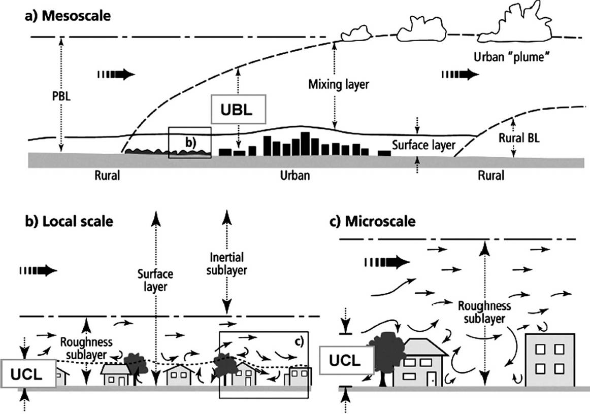
Figure 1: A schematic view of the UHI at multiple scales. (Source)

Models are developed to tackle particular issues related to the UHI. Most models serve a particular purpose and cannot extend to multiple scales of UHI formation. As a result, all scales carry their own share of importance with respect to who in particular is interested. Regardless of personal interest, the UHI in its entirety can only really be understood in a region where all scales have thoroughly been investigated.

Monday 28 November 2016

Modelling Heat Islands - Parameters and Considerations

The Urban Heat Island, similar to most atmospheric phenomenon develops under a set of patterned conditions. It’s highly unlikely that the UHI would form randomly, but the main challenge associated with the UHI is that the conditions for formation are not easily quantifiable. 

In order to model a phenomenon, a thorough understanding of the characteristics of formation is required as the parameters that need to be incorporated into the model are highly dependant on them. Additionally, the conditions for mitigation or UHI decay also need to be understood as they should not be overlooked. Essentially, conditions for formation and depletion are two sides of the same coin, just sitting on opposite extremes. 

To date, the most important meteorological characteristics that have been determined to influence the UHI (positively or negatively) include:


The reason WVC and RH are treated as two separate meteorological conditions is because there is a considerable difference in how the UHI responds to the actual vapour content of the atmosphere and simply how close the system is to saturation, irrespective of the vapour required for it to reach saturation. Regardless of the vapour content, the UHI appears to respond more strongly to how close the system is to saturation. This has not been tested in very warm regions and hence the effect of a very large water vapour content under average RH is still uncertain, which is why it is being considered.

It may seem that these conditions differ from Arnfield’s suggestions for UHI formation and that is particularly because Arnfield dealt primarily with optimising UHI formation whereas in the case of models, we are dealing with all parameters that have been shown to exhibit some form of influence on the UHI. 

Nocturnal UHI Statistical Model in Hamburg (Hoffmann et al., 2011)


A good example of a model developed to model the nocturnal UHI in relation to meteorological conditions is that of Hoffmann et al. (2011) in Hamburg. They worked to model the UHI whereby the parameters would be identified through the use of a generalised least squares method to form a statistical model. To identify the significant meteorological variables to include in their model, a regression based statistical model was developed to test each meteorological condition (X) under a 2-tailed t-test. The explained variance of R^2 was then used to test the strength of the relationship.

 Tu−r =  aX + b

Note: Tu−r refers to UHI intensity (Urban - Rural)

They concluded the most influential conditions were:

  • Wind speed (Negative correlation) ~ This was discussed in a previous post (2 posts ago)
  • Cloud coverage (Negative correlation)
  • Relative Humidity (RH) (Positive correlation)

Wind was found to replace the air within the system, hence weakening the UHI. Cloud coverage prevented escaping heat from cooling the rural region, which then lowered the contrast between the urban and rural stations. High relative humidity meant more vapour would condense in the upper atmosphere releasing latent heat.

They decided to exclude the effects of WVC and Atmospheric pressure due to their observed weak influence on system as part of the study.
  • Water vapour content (WVC) (0.2%)
  • Atmospheric pressure (7.6%)

The linear regression model was then constructed:

Tu−r = aFF + bCC + cRH + d

Whereby:

FF = Windspeed
CC = Cloud Coverage
RH = Relative Humidity

a, b, c, d are fixed parameters to be determined through the least squares method.

The datasets used with respect to the meteorological observations were obtained from the German Meteorological Service (DWD), ERA40 and Regional Climate Model (RCM) results.

The figure below illustrates a frequency distribution of the UHI observed within Hamburg vs values calculated through the model. It was suggested within the paper that the overestimation of UHI was likely due to overestimations in the cloud coverage and relative humidity datasets that were obtained. Additionally, calibrations would need to be made to filter some of the biases in the system. Another factor to consider if applying a model such as this to future climates is the effect of increases in unstable climatic conditions that would rise due to warmer climates.

Figure 1: A frequency distribution plot of observed (Black Asterisk) and modelled UHI intensity using measurements (Black points) and ERA40 (Grey points) for the period of 1985 - 1999. Error bars indicate 95% confidence intervals due to unexplained variance. 


I highly recommend giving this paper a read for a more in depth understanding of the model’s design, capabilities and application. It should be noted that this is a city-scale model, which is ideal for contribution to climate models when appropriate. UHIs also form at smaller scales, each with their own set of approaches and challenges, which will be discussed in the next post. 


Probably...